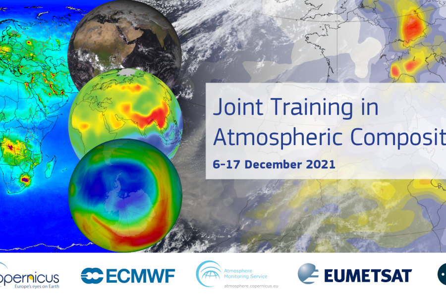
Ensembles are run to account for uncertainties in initial conditions. This lesson explores the sources of error in NWP, how they are quantified, and how ensembles are evaluated.
In this notebook we show a practical example on how to investigate ozone products from the [CDS](https://cds.climate.copernicus.eu/datasets/satellite-ozone-v1?tab=overv…). We will explore here the spatial and temporal ozone distribution of the total ozone columns. Total colum means here, the sum...
Web services are used to visualise geographical data. This lesson describes web services, data standards and outlines what OGC and INSPIRE are.
This notebook-tutorial provides an introduction to the use of the
There are times when consecutive forecasts can 'jump' significantly. This lesson will discuss the ways in which forecast jumpiness can appear and how it can be mitigated.
This lesson guides users through an adaptation case study of an (imaginary) olive farmer in Spain. The lesson contains clips that show how to use and adapt scripts in the toolbox.
This is a Jupyter Notebook (JN) illustrating how to access and use a satellite-derived Greenhouse Gas (GHG) atmospheric carbon dioxide (CO2) Level 2 data product as generated via the Copernicus Climate Change Service (C3S) and made available via the Copernicus Climate Data Store [CDS](https://cds...